Which Language To Use For Data Cleaning

This article was published as a part of the Data Science Blogathon

Introduction

Python is an piece of cake-to-learn programming language, which makes it the nigh preferred choice for beginners in Data Science, Data Analytics, and Car Learning. It also has a smashing community of online learners and excellent data-centric libraries.

With so much information being generated, information technology becomes of import that the data nosotros utilize for Data Science applications like Automobile Learning and Predictive Modeling is make clean. Only what exercise we mean by clean data? And what makes information muddy in the first identify?

Dirty data only means data that is erroneous. Duplicacy of records, incomplete or outdated information, and improper parsing tin make data dirty. This information needs to be cleaned. Information cleaning (or data cleansing) refers to the procedure of "cleaning" this muddy data, by identifying errors in the information then rectifying them.

Data cleaning is an important step in and Machine Learning projection, and we will embrace some basic data cleaning techniques (in Python) in this article.

Cleaning Information in Python

We will learn more about data cleaning in Python with the assistance of a sample dataset. We volition utilise the Russian housing dataset on Kaggle.

Nosotros will first by importing the required libraries.

# import libraries import pandas as pd import numpy as np import seaborn equally sns import matplotlib.pyplot as plt %matplotlib inline

Download the data, and and then read it into a Pandas DataFrame by using the read_csv() part, and specifying the file path. So use the shape attribute to check the number of rows and columns in the dataset. The lawmaking for this is as below:

df = pd.read_csv('housing_data.csv') df.shape

The dataset has 30,471 rows and 292 columns.

Nosotros will now separate the numeric columns from the categorical columns.

# select numerical columns df_numeric = df.select_dtypes(include=[np.number]) numeric_cols = df_numeric.columns.values # select non-numeric columns df_non_numeric = df.select_dtypes(exclude=[np.number]) non_numeric_cols = df_non_numeric.columns.values

We are now through with the preliminary steps. Nosotros can now move on to data cleaning. We volition showtime by identifying columns that comprise missing values and try to fix them.

Missing values

We will commencement by calculating the percentage of values missing in each column, and then storing this information in a DataFrame.

# % of values missing in each column values_list = list() cols_list = list() for col in df.columns:     pct_missing = np.mean(df[col].isnull())*100     cols_list.suspend(col)     values_list.append(pct_missing) pct_missing_df = pd.DataFrame() pct_missing_df['col'] = cols_list pct_missing_df['pct_missing'] = values_list

The DataFrame pct_missing_df at present contains the percent of missing values in each cavalcade along with the column names.

Nosotros can also create a visual out of this data for better understanding using the code below:

pct_missing_df.loc[pct_missing_df.pct_missing > 0].plot(kind='bar', figsize=(12,8)) plt.show()

The output later on execution of the above line of lawmaking should look like this:

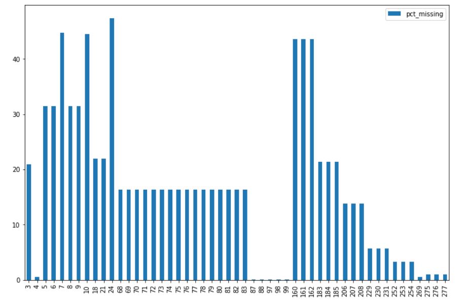
It is articulate that some columns accept very few values missing, while other columns accept a substantial % of values missing. Nosotros will now fix these missing values.

At that place are a number of means in which nosotros tin can prepare these missing values. Some of them are"

Drop observations

One mode could exist to drib those observations that contain any null value in them for any of the columns. This will piece of work when the percent of missing values in each column is very less. We will drop observations that incorporate zilch in those columns that take less than 0.5% nulls. These columns would be metro_min_walk, metro_km_walk, railroad_station_walk_km, railroad_station_walk_min, and ID_railroad_station_walk.

less_missing_values_cols_list = list(pct_missing_df.loc[(pct_missing_df.pct_missing < 0.5) & (pct_missing_df.pct_missing > 0), 'col'].values) df.dropna(subset=less_missing_values_cols_list, inplace=True)

This will reduce the number of records in our dataset to 30,446 records.

Remove columns (features)

Another way to tackle missing values in a dataset would exist to driblet those columns or features that have a pregnant percentage of values missing. Such columns don't contain a lot of information and tin exist dropped altogether from the dataset. In our example, let us drop all those columns that have more than 40% values missing in them. These columns would exist build_year, state, hospital_beds_raion, cafe_sum_500_min_price_avg, cafe_sum_500_max_price_avg, and cafe_avg_price_500.

# dropping columns with more than than xl% nothing values _40_pct_missing_cols_list = list(pct_missing_df.loc[pct_missing_df.pct_missing > 40, 'col'].values) df.drib(columns=_40_pct_missing_cols_list, inplace=True)

The number of features in our dataset is at present 286.

Impute missing values

There is still missing information left in our dataset. We will now impute the missing values in each numerical column with the median value of that column.

df_numeric = df.select_dtypes(include=[np.number]) numeric_cols = df_numeric.columns.values for col in numeric_cols:     missing = df[col].isnull()     num_missing = np.sum(missing)     if num_missing > 0:  # impute values but for columns that take missing values         med = df[col].median() #impute with the median         df[col] = df[col].fillna(med)

Missing values in numerical columns are now fixed. In the case of chiselled columns, we will replace missing values with the mode values of that column.

df_non_numeric = df.select_dtypes(exclude=[np.number]) non_numeric_cols = df_non_numeric.columns.values for col in non_numeric_cols:     missing = df[col].isnull()     num_missing = np.sum(missing)     if num_missing > 0:  # impute values only for columns that accept missing values         mod = df[col].describe()['top'] # impute with the most frequently occuring value         df[col] = df[col].fillna(modern)

All missing values in our dataset have now been treated. We can verify this by running the post-obit piece of lawmaking:

df.isnull().sum().sum()

If the output is goose egg, it means that there are no missing values left in our dataset now.

We tin as well supervene upon missing values with a item value (like -9999 or 'missing') which will indicate the fact that the information was missing in this place. This tin be a substitute for missing value imputation.

Outliers

An outlier is an unusual observation that lies away from the majority of the information. Outliers can affect the operation of a Machine Learning model significantly. Hence, it becomes important to identify outliers and care for them.

Let united states of america take the 'life_sq' column equally an example. Nosotros will outset employ the depict() method to wait at the descriptive statistics and meet if we can get together whatsoever information from it.

df.life_sq.depict()

The output volition await like this:

count    30446.000000 mean        33.482658 std         46.538609 min          0.000000 25%         22.000000 50%         30.000000 75%         38.000000 max       7478.000000 Name: life_sq, dtype: float64

From the output, information technology is clear that something is not right. The max value seems to be abnormally large compared to the hateful and median values. Let us brand a boxplot of this information to go a better idea.

df.life_sq.plot(kind='box', figsize=(12, eight)) plt.show()

The output will look like this:

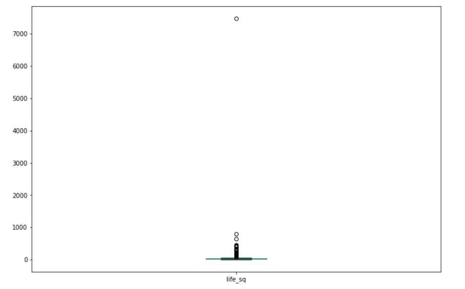
It is articulate from the boxplot that the ascertainment respective to the maximum value (7478) is an outlier in this data. Descriptive statistics, boxplots, and scatter plots help us in identifying outliers in the information.

We can deal with outliers simply like we dealt with missing values. We can either drop the observations that we call up are outliers, or we can supersede the outliers with suitable values, or we tin can perform some sort of transformation on the data (like log or exponential). In our example, let u.s. drop the record where the value of 'life_sq' is 7478.

# removing the outlier value in life_sq column df = df.loc[df.life_sq < 7478]

Duplicate records

Information tin sometimes contain indistinguishable values. It is of import to remove duplicate records from your dataset before you continue with any Machine Learning projection. In our data, since the ID cavalcade is a unique identifier, we will drib duplicate records past because all but the ID column.

# dropping duplicates past because all columns other than ID cols_other_than_id = listing(df.columns)[1:] df.drop_duplicates(subset=cols_other_than_id, inplace=True)

This will aid us in dropping the indistinguishable records. By using the shape method, you can bank check that duplicate records have actually been dropped. The number of observations is thirty,434 at present.

Fixing information type

Frequently in the dataset, values are not stored in the correct data blazon. This can create a problem in afterward stages, and we may non become the desired output or may get errors while execution. Ane mutual information blazon mistake is with dates. Dates are oft parsed as objects in Python. There is a carve up data type for dates in Pandas, chosen DateTime.

We will first cheque the data blazon of the timestamp column in our data.

df.timestamp.dtype

This returns the data type 'object'. Nosotros now know the timestamp is not stored correctly. To set this, let's convert the timestamp column to the DateTime format.

# converting timestamp to datetime format df['timestamp'] = pd.to_datetime(df.timestamp, format='%Y-%m-%d')

We now accept the timestamp in the right format. Similarly, there can be columns where integers are stored every bit objects. Identifying such features and correcting the data type is of import earlier y'all proceed on to Machine Learning. Fortunately for us, we don't take any such issue in our dataset.

EndNote

In this article, nosotros discussed some basic ways in which we can clean data in Python before starting with our Machine Learning project. We need to place and remove missing values, place and treat outliers, remove duplicate records, and set up the data type of all columns in our dataset before we go along with our ML task.

The writer of this article is Vishesh Arora. You can connect with me on LinkedIn.

The media shown in this article on Sign Language Recognition are non owned by Analytics Vidhya and are used at the Writer'due south discretion.

Source: https://www.analyticsvidhya.com/blog/2021/06/how-to-clean-data-in-python-for-machine-learning/

Posted by: smithstord1954.blogspot.com

Share this post